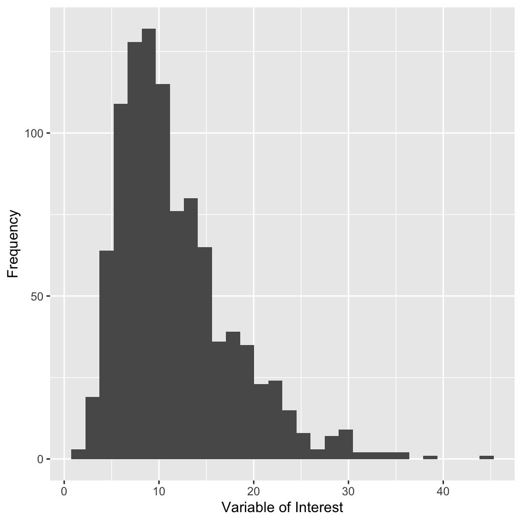
Histograms: Base graphics
- The workhorse function is
hist
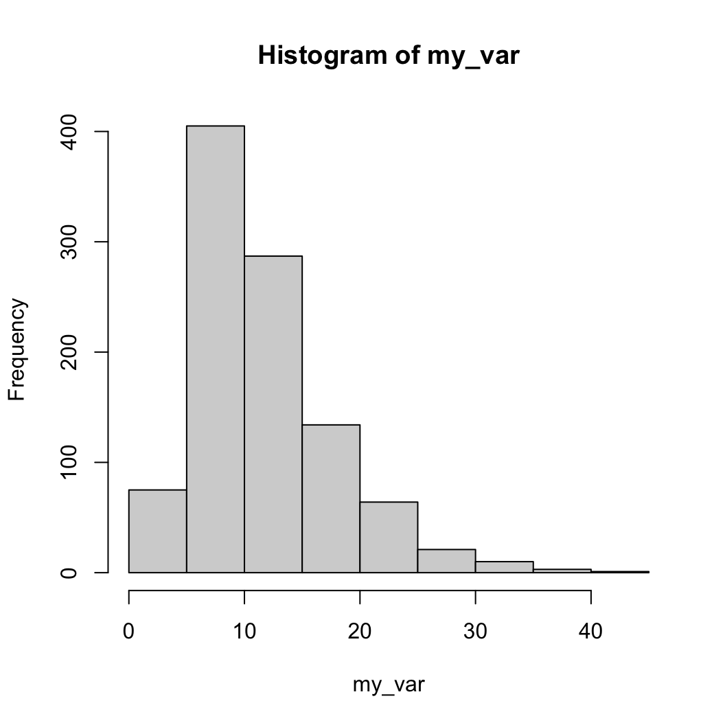
hist
histThe defaults are not very nice, so lets improve things
main = "" disables the titlexlab and ylab control axis labelsbreaks controls the number of bins in the
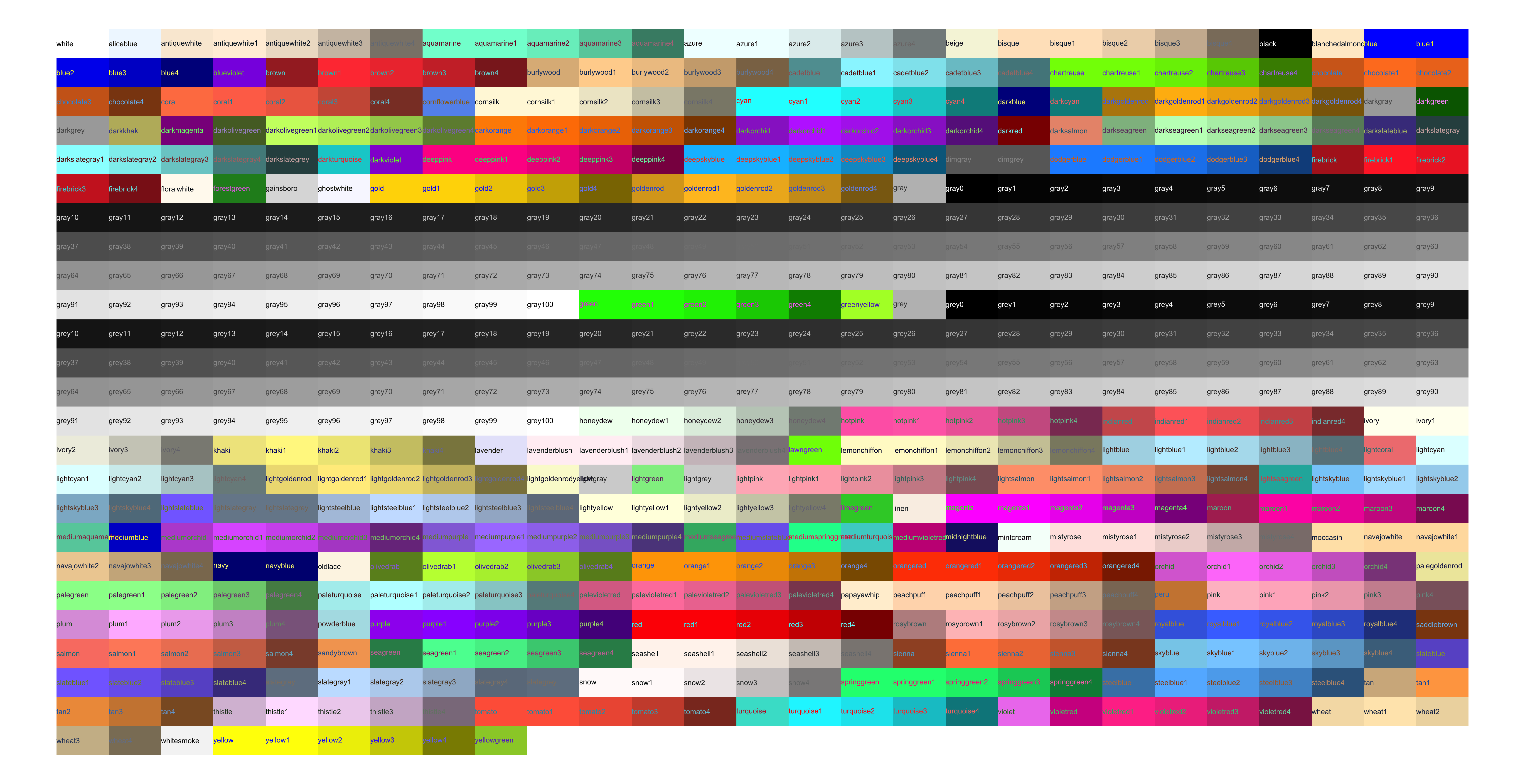
histogramcol sets the color of the barsborder sets the color of the borders (NA:
no border)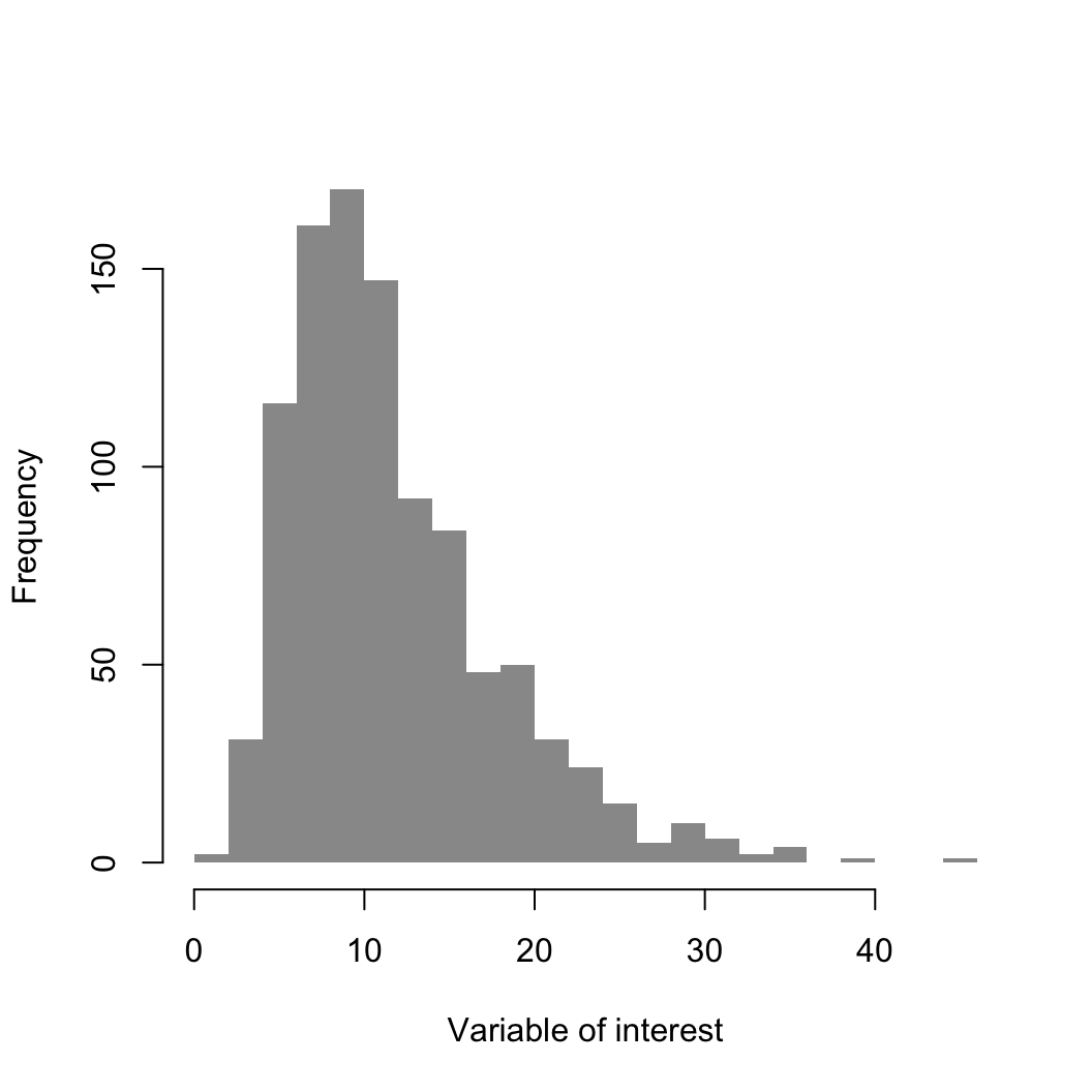
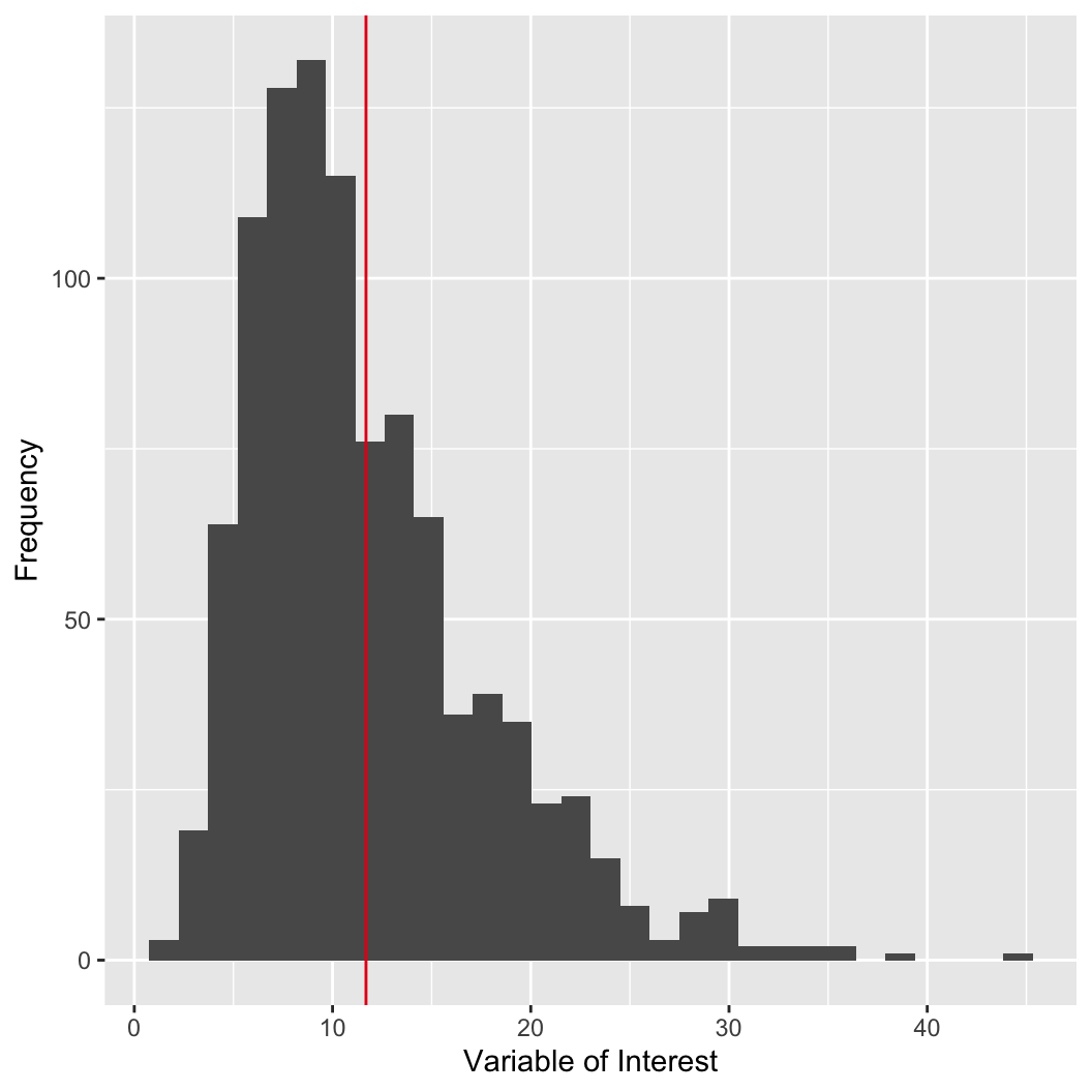
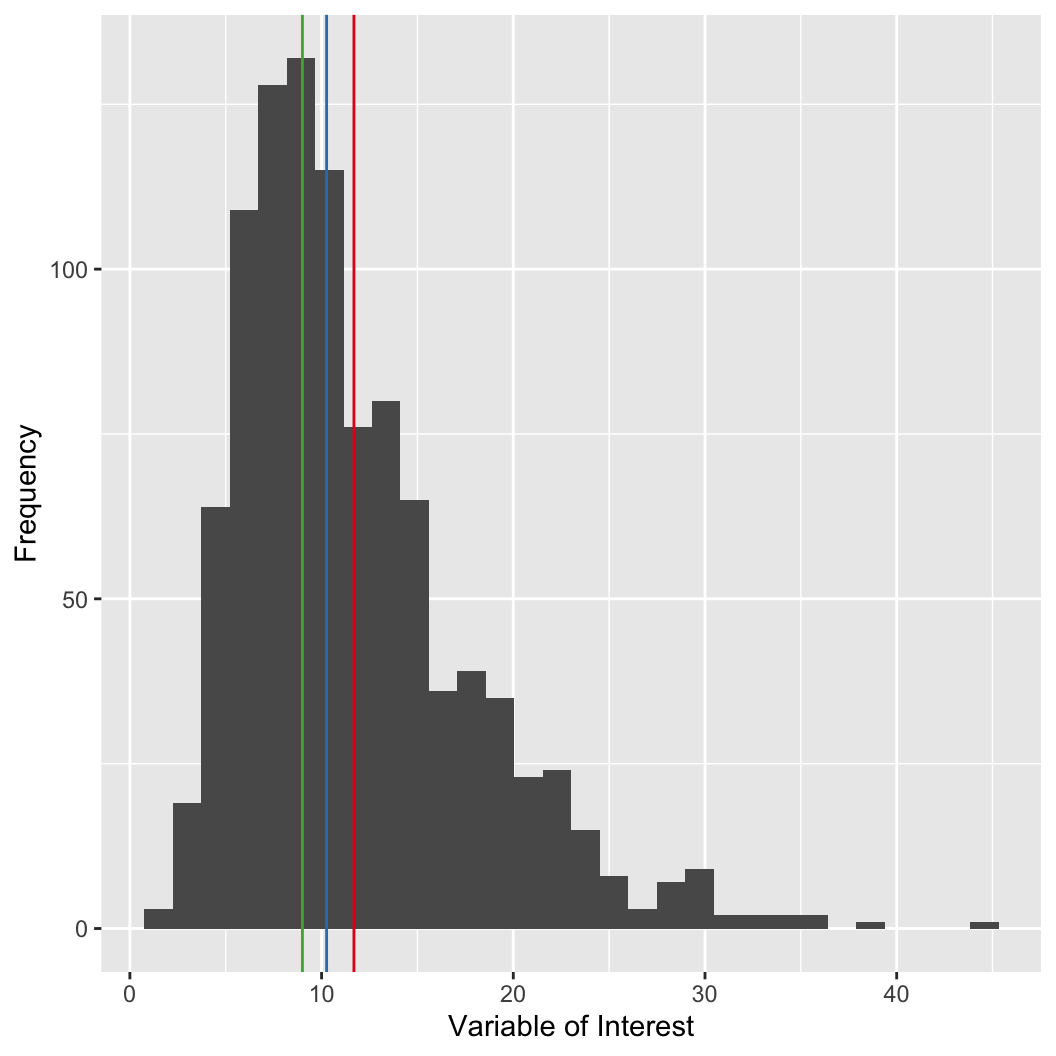
The population mean (\(\mu\)) can be approximated with the sample mean:
\[ \mu \approx \bar{x} = \frac{1}{n}\sum_{i=1}^n x_i \]
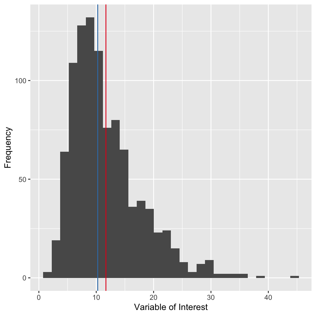
The mean can be strongly influenced by outliers.
The mean can be strongly influenced by outliers.
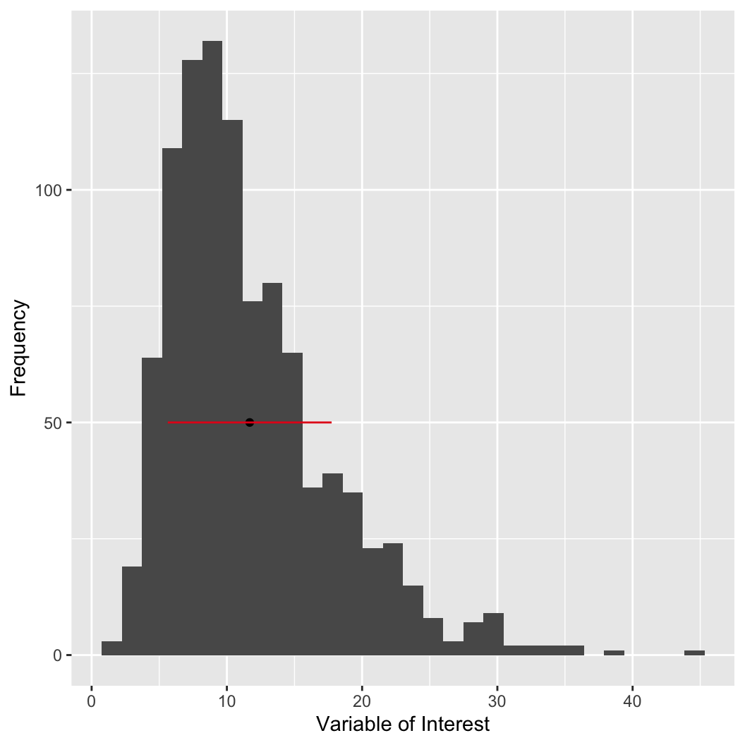
\[ \sigma^2 = \frac{1}{N}\sum_{i=1}^N (X_i-\mu)^2 \]
We can estimate \(\sigma^2\) using the sample variance:
\[ \sigma^2 \approx s^2 = \frac{1}{n-1}\sum_{i=1}^n (x_i -\bar{x})^2 \]
It is convenient to talk about the scale of \(x\) in the same units as \(x\) itself, so we use the (population or sample) standard deviation:
\[ \sigma = \sqrt{\sigma^2} \approx s = \sqrt{s^2} \]
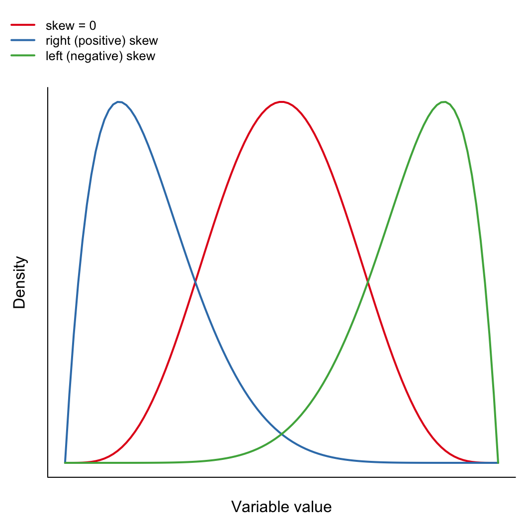
Is the distribution weighted to one side or the other?
\[ \mathrm{skewness} = \frac{\sum_{i=1}^{n}(x_i-\bar{x})^3}{(n-1)s^3} \]
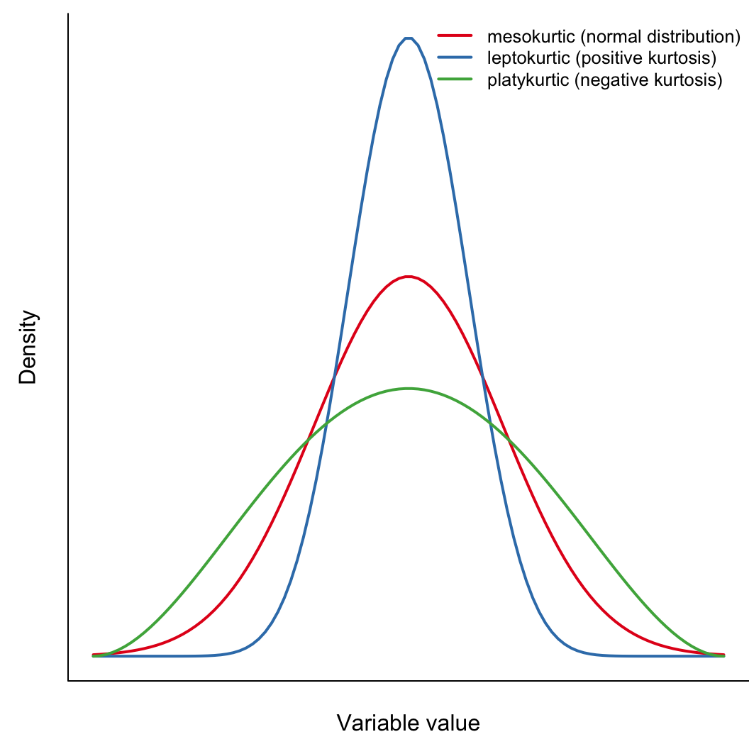
How fat are the tails relative to a normal distribution?
\[ \mathrm{kurtosis} = \frac{\sum_{i=1}^{n}(x_i-\bar{x})^4}{(n-1)s^4} \]
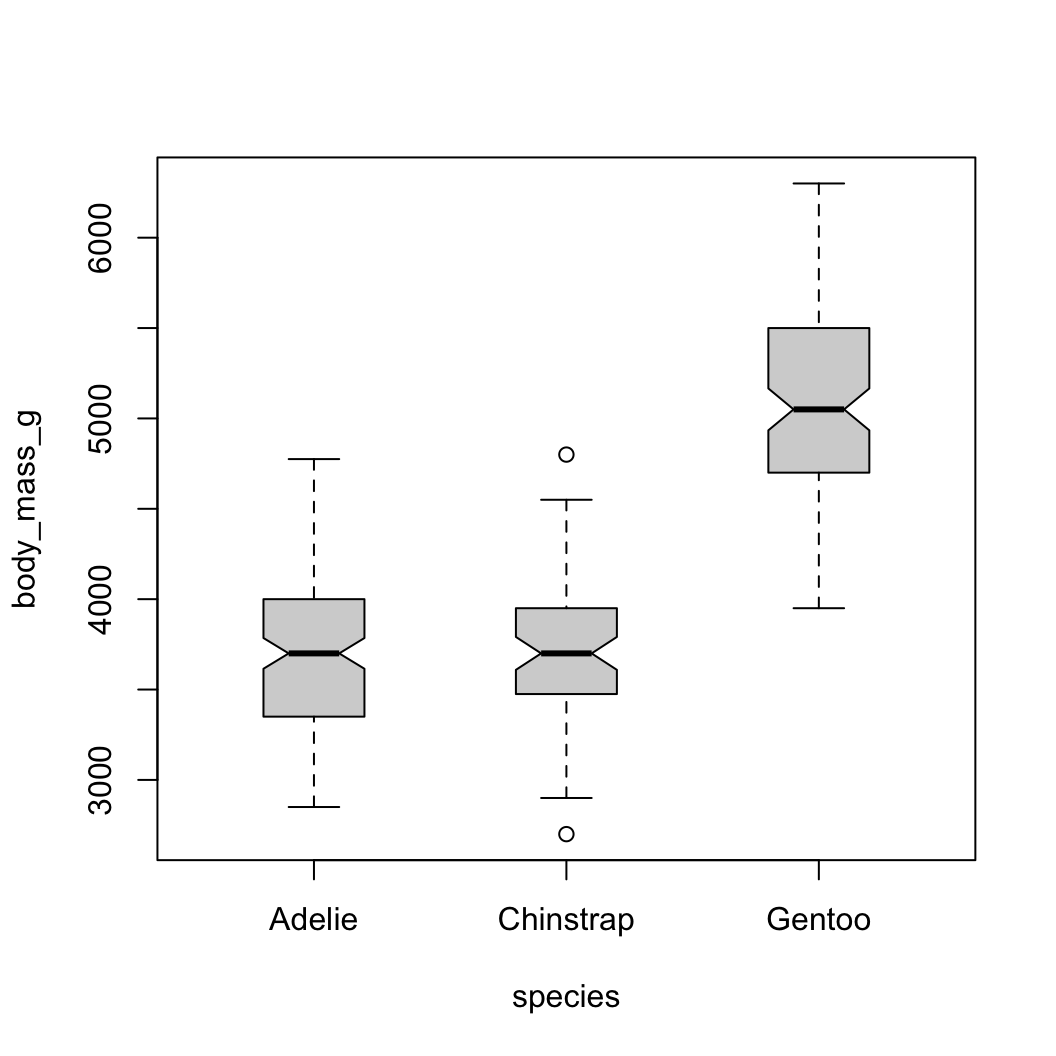
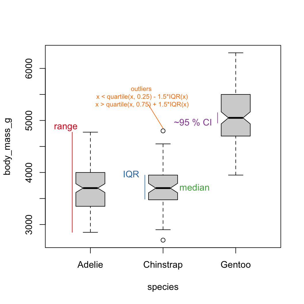
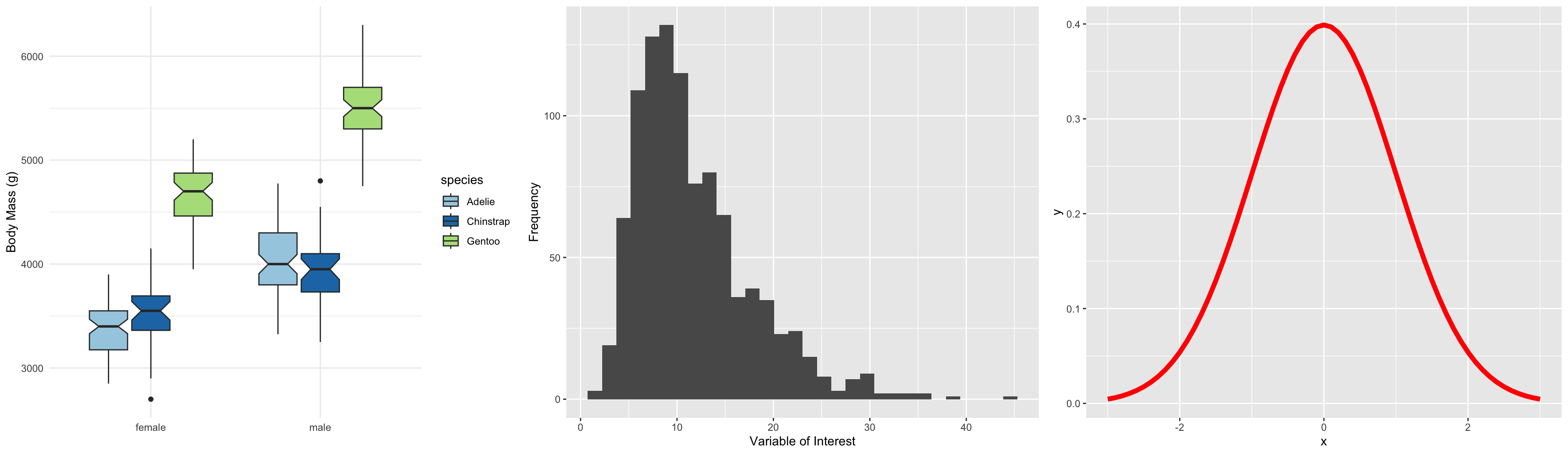
boxplot functiony ~ group is a special data type called a
formulaboxplot functiony ~ group is a special data type called a
formulaboxplot functiony ~ group is a special data type called a
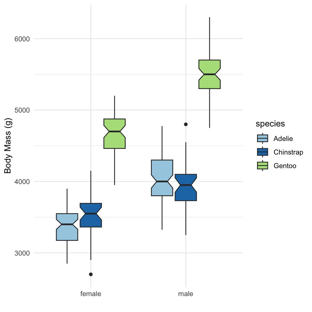
formulaFor more complex groupings, better to use ggplot
Thought experiment
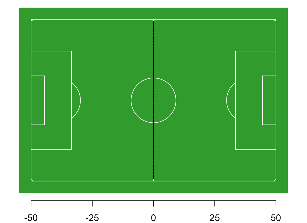
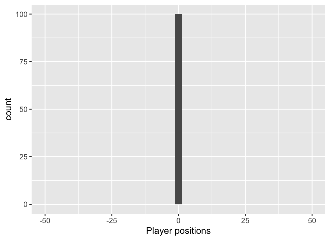
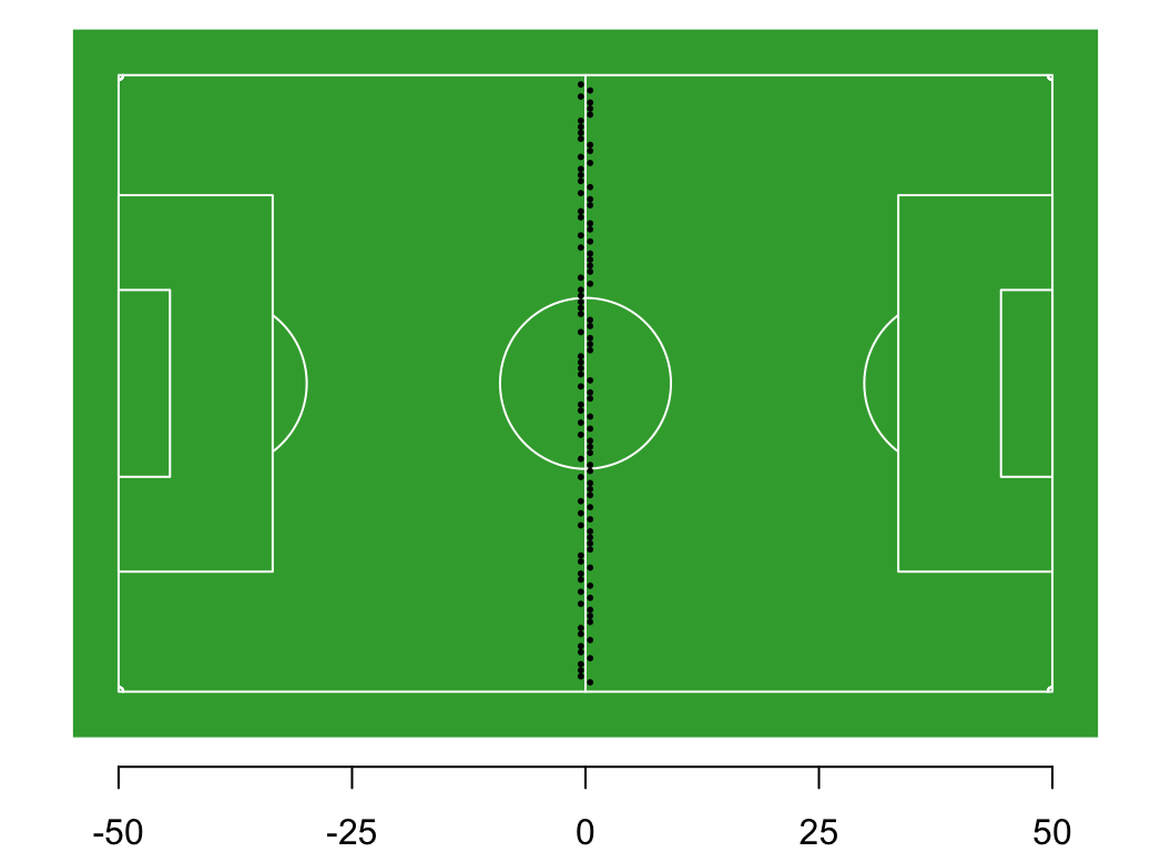
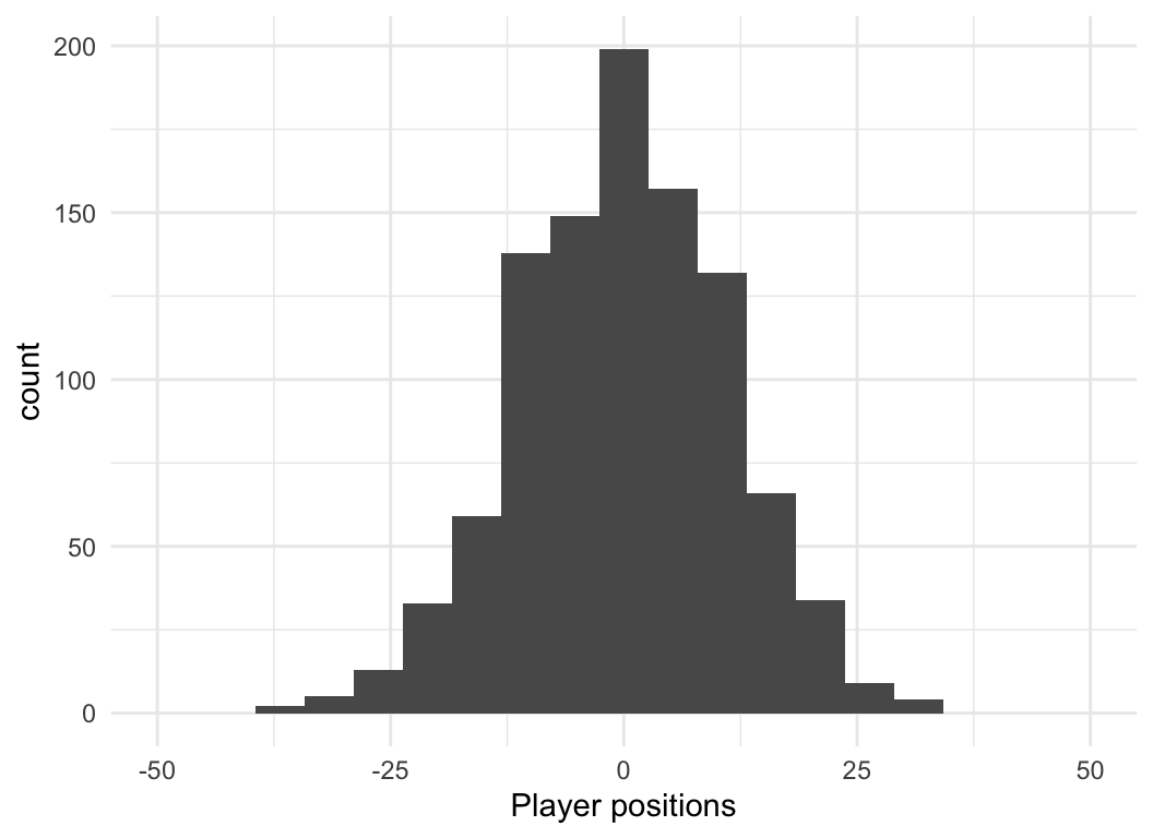
You and 99 of your closest friends gather on the centre line of a 100-m football pitch. We define the centre line as 0m, the western boundary -50 m, and the eastern boundary as +50 m.
Thought experiment
You and 99 of your closest friends gather on the centre line of a 100-m football pitch. We define the centre line as 0m, the western boundary -50 m, and the eastern boundary as +50 m.
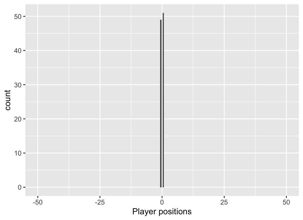
Each person flips a coin. If the coin is heads, they take a step east (add 0.5 m to their location), if its tails, they take a step west (subtract 0.5 m from their location).
Question: What is the long-run distribution of positions on the field?
Thought experiment
You and 99 of your closest friends gather on the centre line of a 100-m football pitch. We define the centre line as 0m, the western boundary -50 m, and the eastern boundary as +50 m.
Each person flips a coin. If the coin is heads, they take a step east (add 0.5 m to their location), if its tails, they take a step west (subtract 0.5 m from their location).
Question: What is the long-run distribution of positions on the field?
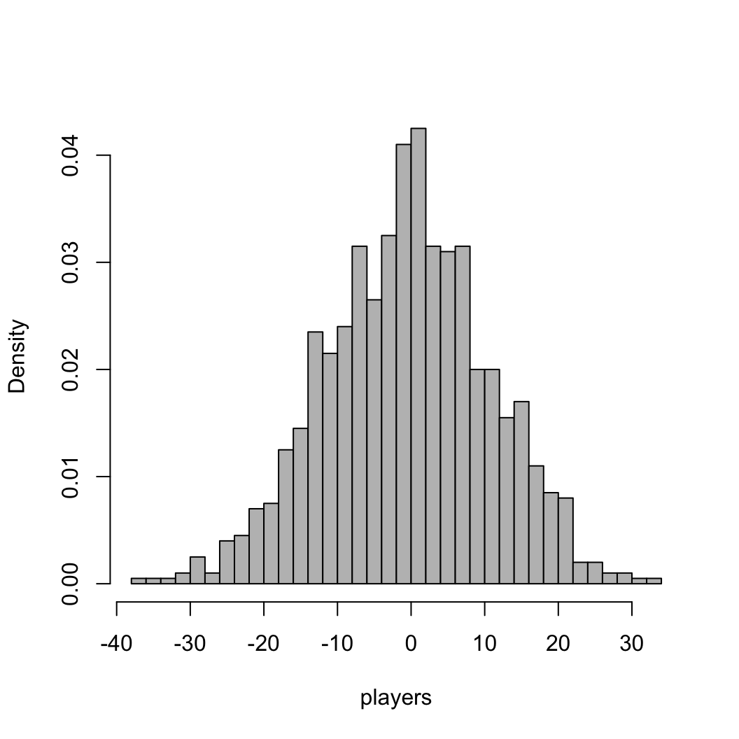
Exercise: Try to simulate this process in R. What does the distribution of locations look like after 10 steps? After 100? What is the long-run distribution with many steps and many players?
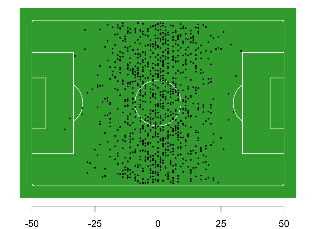
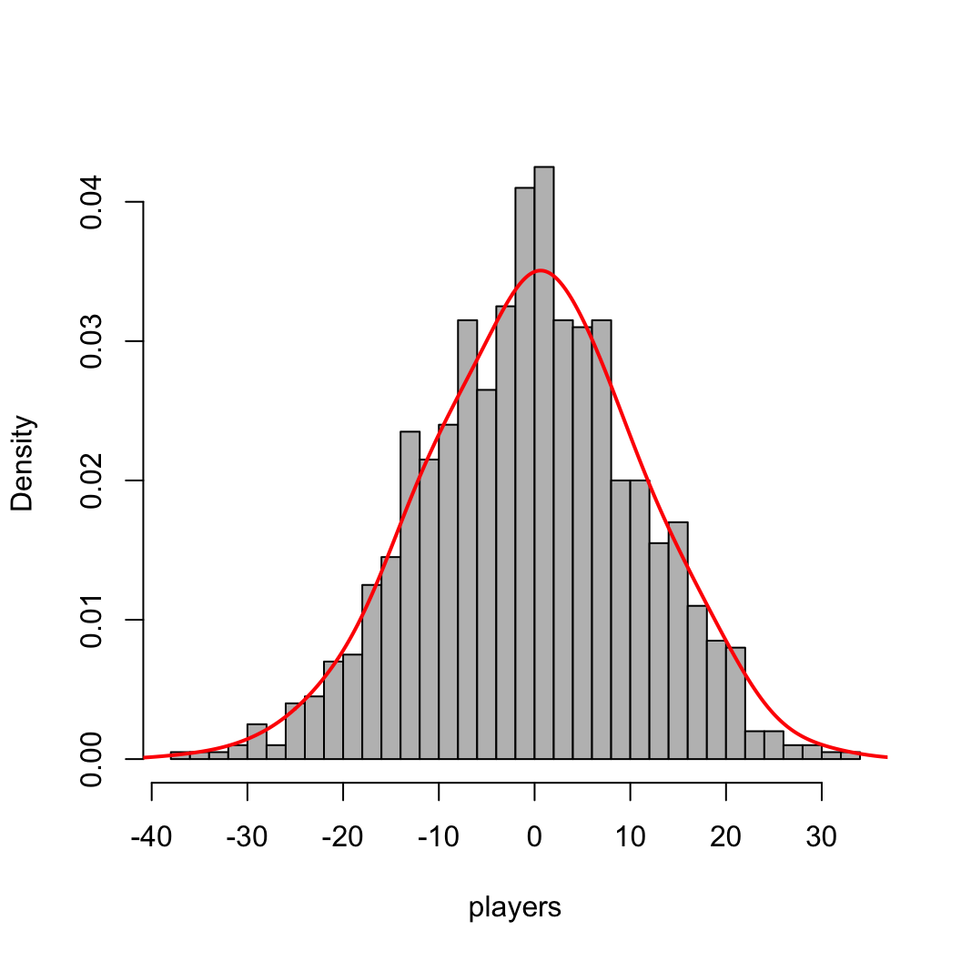
density function in R to add a curve
approximating this density.hist(players, breaks=40, col="gray", main = "", freq=FALSE)
lines(density(players, adjust=1.5), col='red', lwd=2)
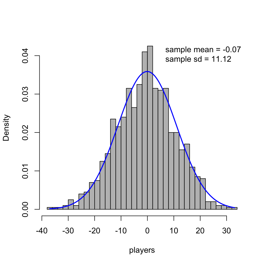
mu = mean(players)
sig = sd(players)
x_norm = seq(min(players), max(players), length.out = 400)
y_norm = dnorm(x_norm, mu, sig)
lines(x_norm, y_norm, lwd=2, col='blue')
legend("topright", legend=c(paste("sample mean =", round(mu, 2)),
paste("sample sd =", round(sig, 2))), lwd=0, bty='n')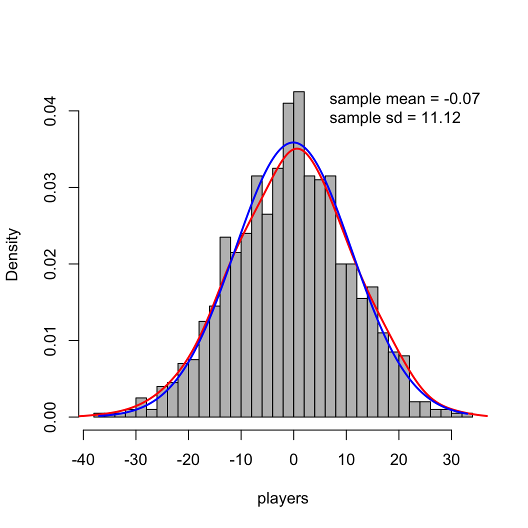
\[ \mathcal{f}(x) = \frac{1}{\sigma \sqrt{2\pi}} \mathcal{e}^{-\frac{1}{2} \left (\frac{x-\mu}{\sigma} \right )^2} \]
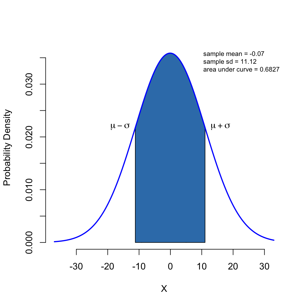
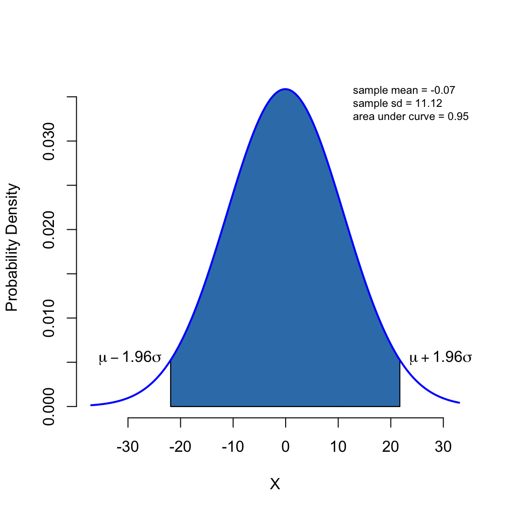
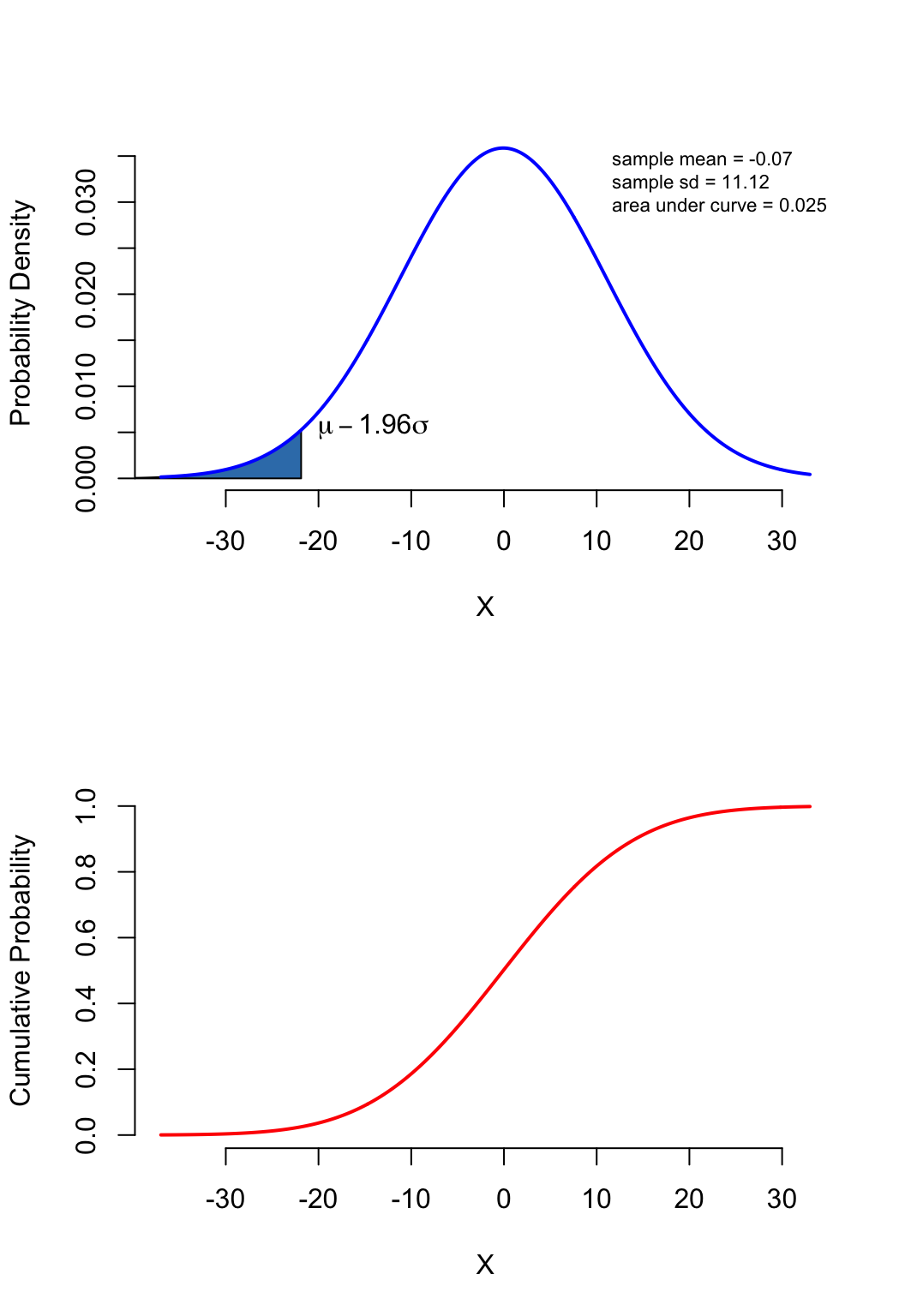
\[ \mathcal{g}(x) = \int_{-\infty}^{x} \frac{1}{\sigma \sqrt{2\pi}} \mathcal{e}^{-\frac{1}{2} \left (\frac{x-\mu}{\sigma} \right )^2} dx \]
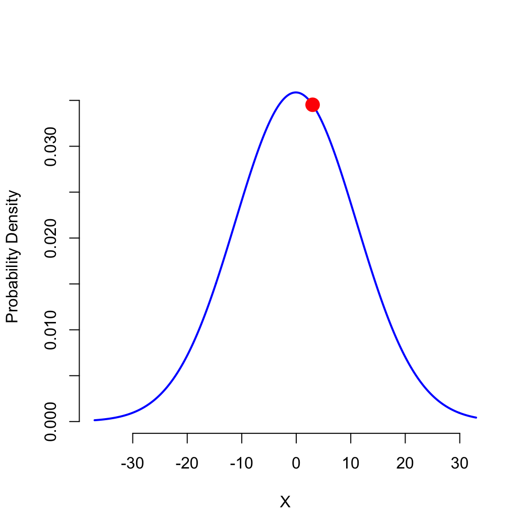
PDF: what is the probability density
when \(x=3\) (the height of the bell
curve)
PDF: what is the probability density
when \(x=3\) (the height of the bell
curve)
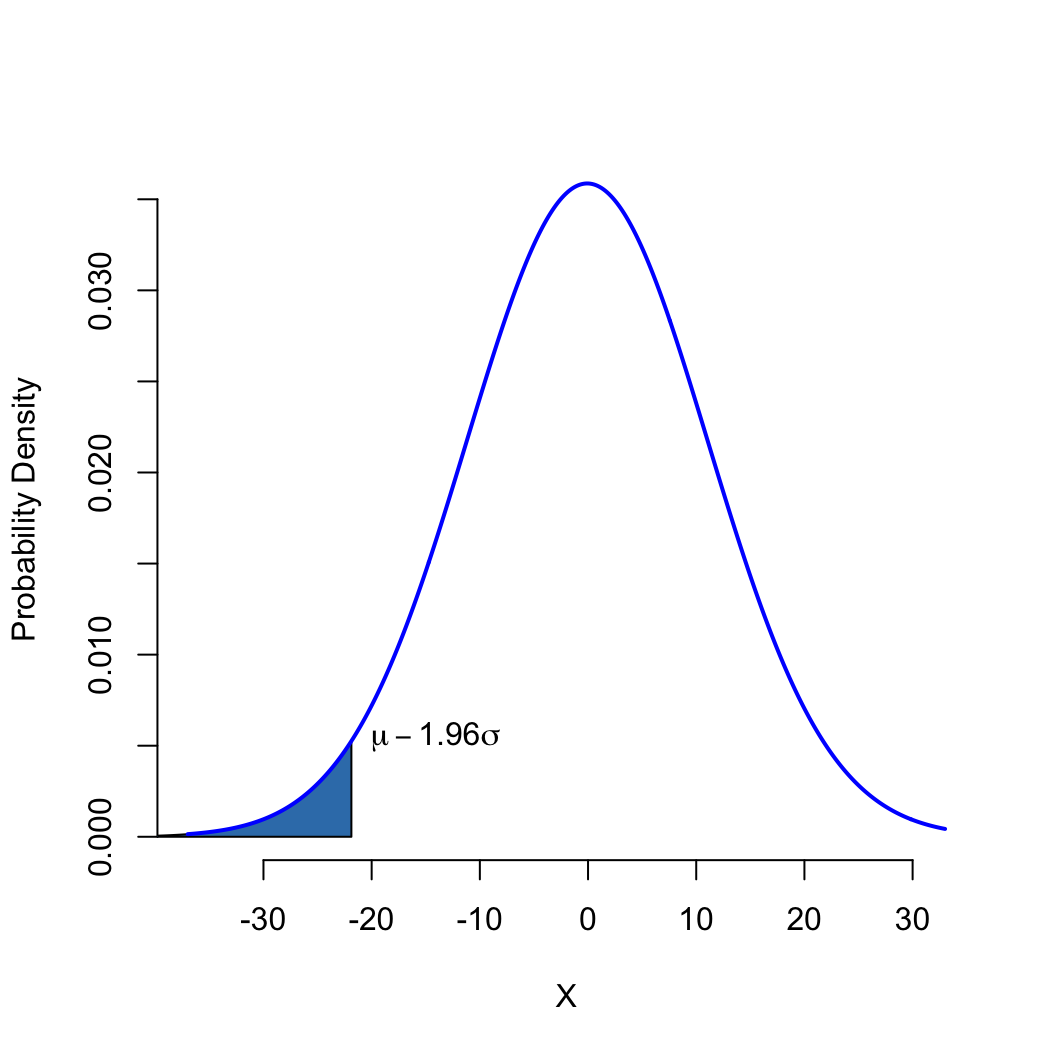
CDF: what is the cumulative probability
when \(x=q\)
(area under the bell curve from \(-\infty\) to \(q\))
(probability of observing a value < \(q\))